Excel worksheets can sometimes get hidden accidentally, making it difficult to access important information. Luckily, there are simple steps you can take to unhide these worksheets and regain access to your data. In this article, we will explore how to unhide Excel worksheets with ease.
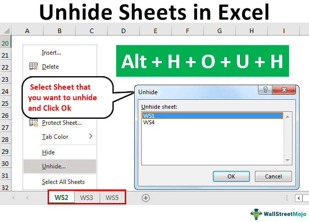
To unhide a worksheet in Excel, you can follow these simple steps:
1. Right-click on any visible worksheet tab: Start by right-clicking on any visible worksheet tab at the bottom of the Excel window. This will bring up a menu with various options.
2. Select “Unhide”: From the menu that appears after right-clicking, select the “Unhide” option. This will show a list of all hidden worksheets in the workbook.
3. Choose the worksheet to unhide: After selecting the “Unhide” option, you will see a list of all hidden worksheets in the workbook. Simply choose the worksheet you want to unhide and click “OK”. The selected worksheet will now be visible again.
4. Repeat if necessary: If you have multiple worksheets that are hidden, you can repeat the above steps to unhide each worksheet individually. This way, you can regain access to all the hidden data in your Excel workbook.
By following these simple steps, you can easily unhide Excel worksheets and access important information without any hassle. Remember to save your changes after unhiding worksheets to ensure that your data is properly secured.
Unhiding Excel worksheets is a simple process that can be done in just a few clicks. By following the steps outlined in this article, you can quickly unhide any hidden worksheets in your Excel workbook and access the data you need. Don’t let hidden worksheets prevent you from working efficiently in Excel – unhide them and get back to work!
